Classifier-free Guidance with Cosine Schedules Pt. 3
diffusion
classifier-free guidance
deep learning
Author
enzokro
Published
November 23, 2022
Experiments with cosine schedules and normalizations for Classifier-free Guidance.
Introduction
This notebook is Part 3 in a series on dynamic Classifier-free Guidance. It combines normalizations and schedules for the guidance parameter \(G\).
Quick recap of Parts 1 and 2
In Part 1, we generated a baseline image using a constant Classifier-free Guidance. Attempting to improve on the baseline, we swept the guidance parameter \(G\) over a set of Cosine Schedules.
In Part 2, we introduced normalizations for Classifier-free Guidance. There was one kind of normalization, Prediction Normalization, that seems to improve the overall quality of generated images.
Part 3: Combining schedules and normalizations
In Part 3, we build on the previous results by now combining guidance normalizations and schedules.
The goal is to find a combo of normalized schedules that universally improve the outputs of Diffusion image models.
Leveraging a few helper libraries
We reuse our helper libraries to more efficiently run guidance experiments. The two libraries are:
import osimport mathimport randomimport warningsfrom PIL import Imagefrom typing import Listfrom pathlib import Pathfrom types import SimpleNamespacefrom fastcore.allimport Lfrom functools import partialimport numpy as npimport matplotlib.pyplot as plt# imports for diffusion modelsimport torchfrom transformers import logging# for clean outputswarnings.filterwarnings("ignore")logging.set_verbosity_error()# set the hardware devicedevice ="cuda"if torch.cuda.is_available() else"mps"if torch.has_mps else"cpu"
2022-11-24 18:34:14.079096: I tensorflow/stream_executor/platform/default/dso_loader.cc:53] Successfully opened dynamic library libcudart.so.11.0
Seed for reproducibility
We use the seed_everything function to make sure that the results are repeatable across notebooks.
# set the seed and pseudo random number generatorSEED =1024def seed_everything(seed): random.seed(seed) os.environ['PYTHONHASHSEED'] =str(seed) np.random.seed(seed) generator = torch.manual_seed(seed) torch.backends.cudnn.deterministic =True torch.backends.cudnn.benchmark =Falsereturn generator# for sampling the initial, noisy latentsgenerator = seed_everything(SEED)
Importing the helper libraries
The cf_guidance library has the guidance schedules and normalizations.
# helpers to create cosine schedulesfrom cf_guidance.schedules import get_cos_sched# normalizations for classifier-free guidancefrom cf_guidance.transforms import GuidanceTfm, BaseNormGuidance, TNormGuidance, FullNormGuidance
The min_diffusion library loads a Stable Diffusion model from the HuggingFace hub.
# to load Stable Diffusion pipelinesfrom min_diffusion.core import MinimalDiffusion# to plot generated imagesfrom min_diffusion.utils import show_image, image_grid, plot_grid
Loading the new openjourney model from Prompt Hero
The following code loads the openjourney Stable Diffusion model on the GPU, with torch.float16 precision.
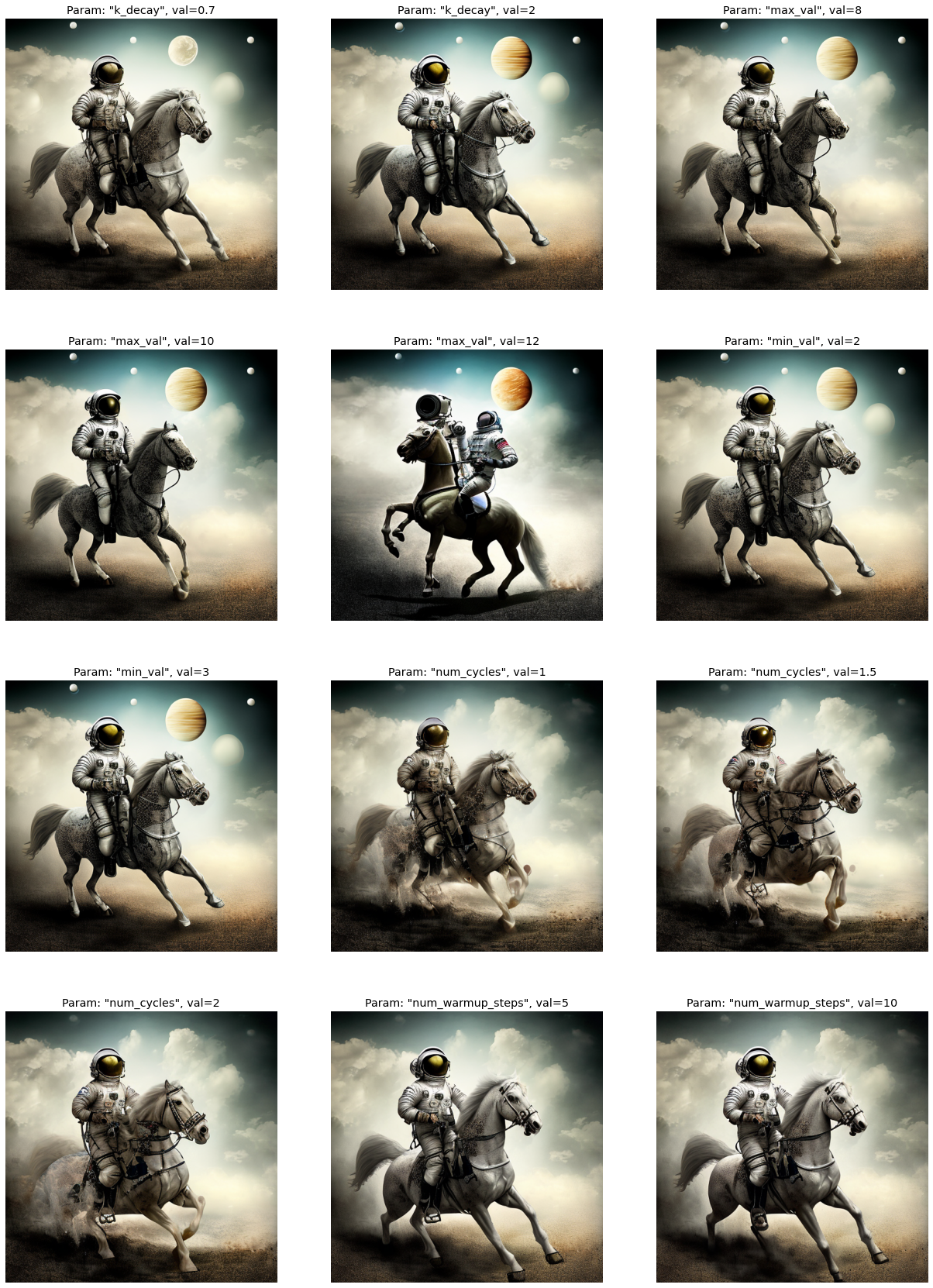
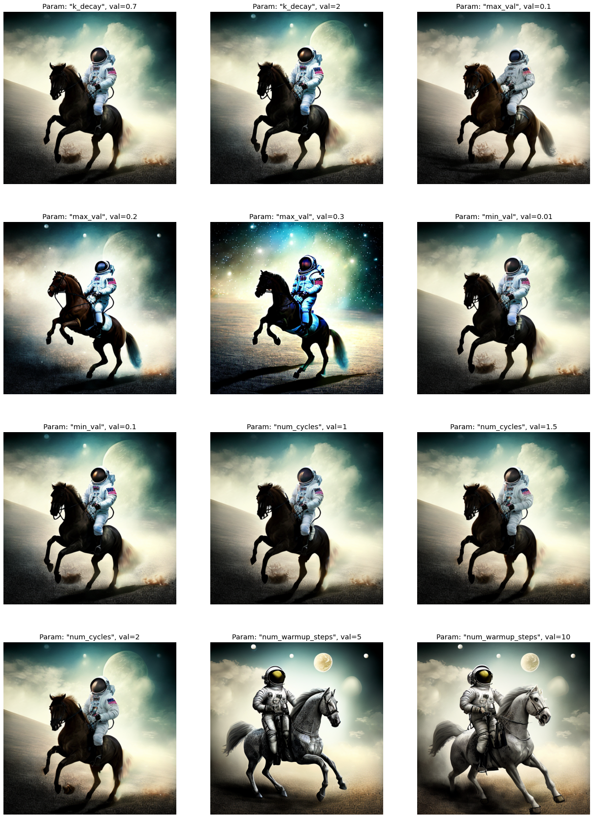
We use the familiar, running prompt in our series to generate an image:
“a photograph of an astronaut riding a horse”
Important
The openjourney model was fine-tuned to create images in the style of Midjourney v4.
To enable this fine-tuned style, we need to add the keyword "mdjrny-v4" at the start of the prompt.
# text prompt for image generationsprompt ="mdjrny-v4 style a photograph of an astronaut riding a horse"
Image parameters
The images will be generated over \(50\) diffusion steps. They will have a height and width of 512 x 512 pixels.
# the number of diffusion stepsnum_steps =50# generated image dimensionswidth, height =512, 512
Function to run the experiments
The run function below generates images for the text prompt.
The function sweeps a given set of schedules using the guidance normalization guide_tfm. It also stores the output images with a matching title for plotting and visualizations.
def run(prompt, schedules, guide_tfm=None, generator=None, show_each=False, test_run=False):"""Runs a dynamic Classifier-free Guidance experiment. Generates an image for the text `prompt` given all the values in `schedules`. Uses a Guidance Transformation class from the `cf_guidance` library. Stores the output images with a matching title for plotting. Optionally shows each image as its generated. If `test_run` is true, it runs a single schedule for testing. """# store generated images and their title (the experiment name) images, titles = [], []# make sure we have a valid guidance transformassert guide_tfmprint(f'Using Guidance Transform: {guide_tfm}')# optionally run a single test scheduleif test_run:print(f'Running a single schedule for testing.') schedules = schedules[:1]# run all schedule experimentsfor i,s inenumerate(schedules):# parse out the title for the current run cur_title = s['title'] titles.append(cur_title)# create the guidance transformation cur_sched = s['schedule'] gtfm = guide_tfm({'g': cur_sched})print(f'Running experiment [{i+1} of {len(schedules)}]: {cur_title}...') img = pipeline.generate(prompt, gtfm, generator=generator) images.append(img)# optionally plot the imageif show_each: show_image(img, scale=1)print('Done.')return {'images': images,'titles': titles,}
The Baseline: Constant Guidance with \(G =7.5\)
Here we create the baseline image. Then we check how the normalized, scheduled guidances change the output.
The baseline Classifier-free Guidance uses a constant update of \(G = 7.5\).
# create the baseline Classifier-free Guidancebaseline_params = {'max_val': [7.5]}# parameters we are sweepingbaselines_names =sorted(list(baseline_params))baseline_scheds = L()# step through each parameterfor idx,name inenumerate(baselines_names):# step through each of its valuesfor idj,val inenumerate(baseline_params[name]):# create the baseline experimeent expt = {'param_name': name,'val': val,'schedule': [val for _ inrange(num_steps)] }# for plotting expt['title'] =f'Param: "{name}", val={val}'# add to the running list of experiments baseline_scheds.append(expt)
We will be creating a lot of experiments, so let’s put this code in a function.
def create_expts(params: dict, schedule_func) ->list: names =sorted(params) expts = []# step through parameter names and their valuesfor i,name inenumerate(names):for j,val inenumerate(params[name]):# create the experiment expt = {'param_name': name,'val': val,'schedule': schedule_func({name: val}),}# name for plotting expt['title'] =f'Param: "{name}", val={val}'# add it to the experiment list expts.append(expt)return expts
# create the baseline schedule with the new functionbaseline_g =7.5baseline_params = {'max_val': [baseline_g]}baseline_func =lambda params: [baseline_g for _ inrange(num_steps)]baseline_expts = create_expts(baseline_params, baseline_func)
Let’s create the baseline image. The hope is that our guidance changes will improve on it.
Using Guidance Transform: <class 'cf_guidance.transforms.GuidanceTfm'>
Running experiment [1 of 1]: Param: "max_val", val=7.5...
Done.
# view the baseline imagebaseline_res['images'][0]
Improving the baseline with schedules and normalizations
This part is similar to its matching sections in Part 1 and Part 2.
Here we create the sweep of Cosine Schedules and the normalizations.
Setting the schedule parameters
Recall that there are three kinds of schedules:
A static schedule with a constant \(G\).
A decreasing Cosine schedule.
A Cosine schedule with some initial warm up steps.
We already created the static schedule 1. in the baseline above. This section creates variations of schedules 2. and 3..
:::: {.callout-note}.
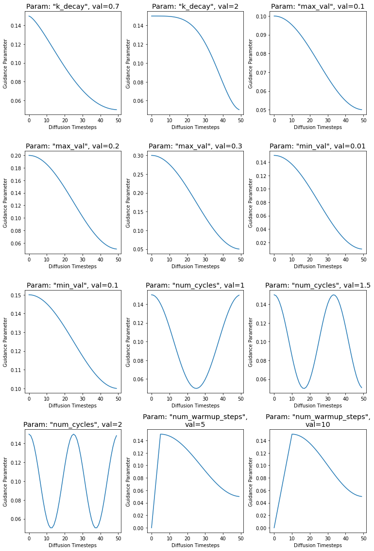
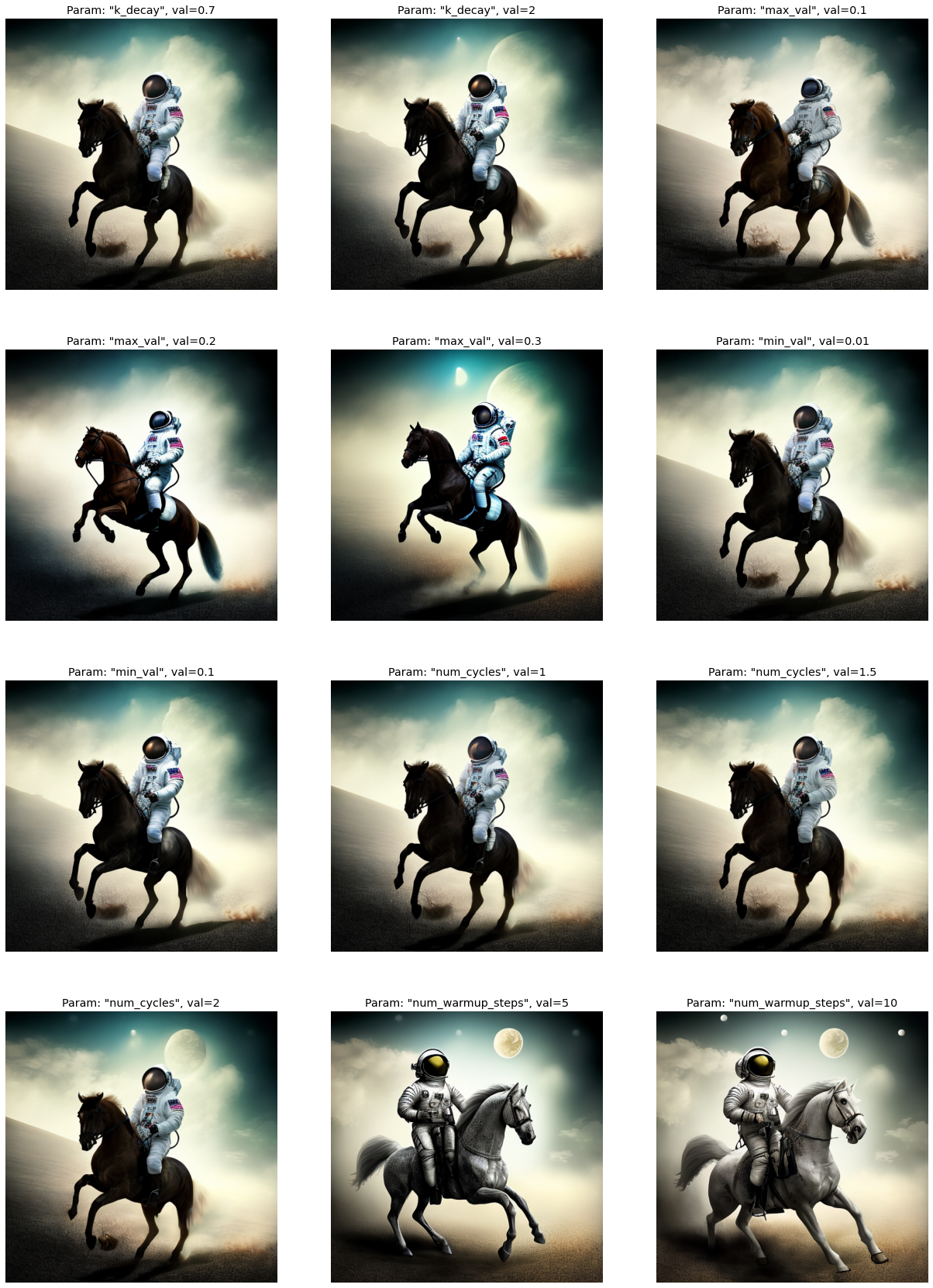
We need smaller guidance values for T-Normalization and Full Normalization.
These normalizations get their own, smaller value of \(G_\text{small} = 0.15\). This smaller value keeps the guidance update vector \(\left( t - u \right)\) from exploding in scale.
::::
# Default schedule parameters from the blog post######################################max_val =7.5# guidance scaling valuemin_val =1# minimum guidance scalingnum_steps =50# number of diffusion stepsnum_warmup_steps =0# number of warmup stepswarmup_init_val =0# the intial warmup valuenum_cycles =0.5# number of cosine cyclesk_decay =1# k-decay for cosine curve scaling # smaller values for T-Norm and FullNormmax_T =0.15min_T =0.05######################################
To make sure our changes always reference this shared starting point, we can wrap these parameters in a dictionary.
We also create a matching dictionary for the T-Norm params.
Every new, incremental schedule will start from these shared dictionaries. Then, a single parameter is changed at a time.
The cos_harness below gives us an easy way of making these minimum-pair changes.
def cos_harness(new_params={}, default_params={}):'''Creates cosine schedules with updated parameters in `new_params` '''# start from the given baseline `cos_params` cos_params =dict(default_params)# update the schedule with any new parameters cos_params.update(new_params)# return the new cosine schedule sched = get_cos_sched(**cos_params)return sched
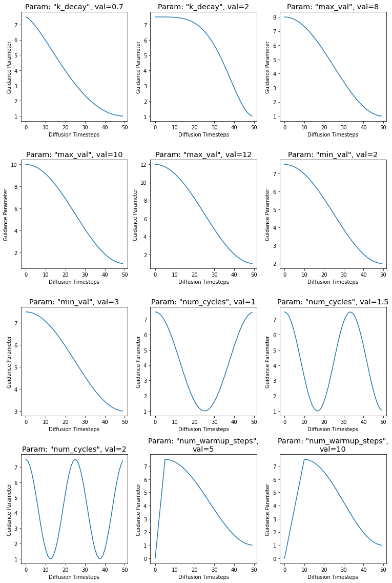
Plotting the Cosine Schedules
Now we create the different Cosine schedules that will be swept.